Bernoulli’s Theorem: Equation, Derivation, and Engineering Applications
Bernoulli’s Theorem is the foundation on which a vast range of fluid engineering calculations are built. From the way a Venturi meter measures flow in an oil and gas pipeline to the lift generated by an aircraft wing, and from the sizing of pressure relief nozzles on ASME-stamped vessels to the analysis of blood flow through a narrowed artery, this single principle — that energy is conserved along a streamline in a flowing fluid — underpins them all. Understanding Bernoulli’s equation in full, including its assumptions, its mathematical derivation, and its real-world limitations, is an essential competency for any engineer working with fluids, piping, or pressure equipment.
This article presents Bernoulli’s Theorem from first principles. It covers the complete mathematical statement, the companion continuity equation, the physical meaning of each term, the assumptions required for valid application, and worked numerical examples. An interactive calculator below lets you solve Venturi meter problems and two-point Bernoulli problems directly. The applications section connects the theorem to the specific instruments and systems encountered in process and industrial engineering.
Bernoulli / Venturi Flow Calculator
Solve two-point Bernoulli problems or calculate Venturi meter flow rate. All inputs in SI units.
Solves for P₂ (pressure at Point 2). Enter all other values.
What Is Bernoulli’s Theorem?
Bernoulli’s Theorem is a statement of the conservation of energy applied to a flowing fluid. It was first formulated by the Swiss mathematician Daniel Bernoulli in his 1738 work Hydrodynamica and later given a rigorous mathematical foundation by Leonhard Euler. The theorem establishes that for an ideal (non-viscous, incompressible) fluid in steady flow, the total mechanical energy per unit volume is the same at every point along a streamline.
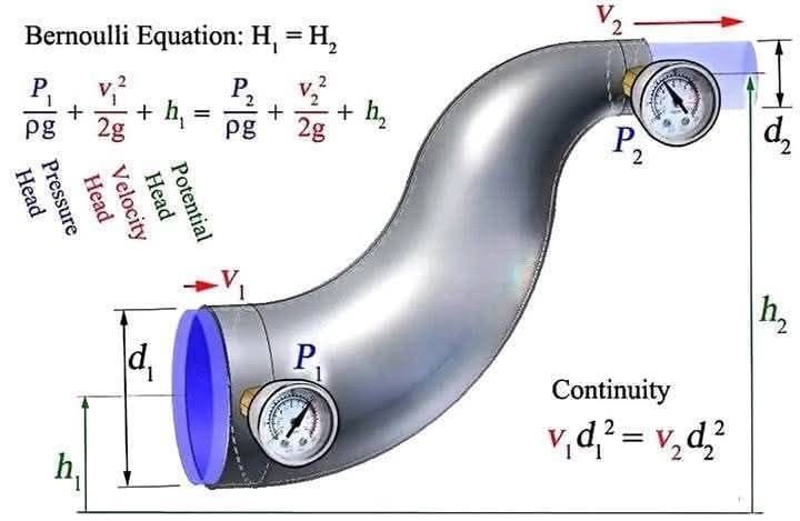
“In a steady, incompressible, inviscid fluid flow, the total energy per unit volume — comprising pressure energy, kinetic energy, and potential energy — remains constant along any streamline.”
P + ½ρv² + ρgh = constant (along a streamline)Written between two points on the same streamline, this becomes the form used in engineering calculations:
The Three Energy Components
Each term in Bernoulli’s equation represents a distinct form of mechanical energy per unit volume. Understanding what each term means physically is the key to applying the equation correctly.
Static Pressure (P)
Static pressure is the actual thermodynamic pressure of the fluid — the force per unit area exerted perpendicular to any surface in contact with the fluid. In a pipe, it is measured by a pressure gauge connected through a wall tap that is perpendicular to the flow direction. Static pressure is the dominant term at low flow velocities. In Bernoulli’s equation, it acts as the “pressure energy” stored in the fluid per unit volume, with units of Pa (N/m²).
Dynamic Pressure (½ρv²)
Dynamic pressure quantifies the kinetic energy of the fluid per unit volume. It is the pressure rise that would occur if the fluid were brought to rest isentropically (without energy loss). The symbol q is often used: q = ½ρv². When flow velocity is high — for example at the throat of a Venturi meter or at the tip of a pitot tube — dynamic pressure is significant. As static pressure falls in a high-velocity zone, dynamic pressure rises by the same amount, keeping the sum constant.
Hydrostatic Pressure (ρgh)
The third term represents gravitational potential energy per unit volume. Elevation h is measured from an arbitrary datum — only differences in h matter, not the absolute value. For horizontal pipelines, h₁ = h₂ and this term cancels, simplifying the equation considerably. For pumped systems that move fluid to higher elevations, this term captures the energy that must be supplied to overcome gravity.
Derivation of Bernoulli’s Equation from Work-Energy Theorem
Bernoulli’s equation can be derived rigorously from Newton’s second law applied to a fluid element (Euler’s equation) or more intuitively from the work-energy theorem. The following derivation uses the work-energy approach and is valid for an incompressible, inviscid fluid in steady flow.
The Continuity Equation — The Essential Companion
Bernoulli’s equation alone is not sufficient to analyse flow in a pipe that changes cross-section. You also need the continuity equation, which expresses conservation of mass. For an incompressible fluid in steady flow:
Together, the continuity equation and Bernoulli’s equation form a two-equation system that allows complete solution of any two-point incompressible flow problem: if you know flow rate, pipe diameters, elevations, and one pressure, you can find the other pressure — and vice versa. This is exactly what a Venturi meter exploits: the known geometry (d₁ and d₂) and a measured pressure difference yield the unknown flow rate.
Flow Through a Converging Pipe: Pressure and Velocity Distribution
Assumptions and Limitations of Bernoulli’s Equation
Bernoulli’s equation in its standard form is derived under idealised conditions. In real engineering systems, these assumptions are rarely met exactly, and engineers must know when corrections are needed.
| Assumption | What It Means | When It Breaks Down | Engineering Correction |
|---|---|---|---|
| Steady flow | Flow properties at each point are constant in time | Start-up/shutdown, pulsating flow, water hammer | Unsteady Bernoulli with ∂v/∂t term |
| Incompressible fluid | Density ρ is constant | Gas flow at Mach > 0.3; steam; compressors | Compressible flow equations |
| Inviscid (no friction) | No viscous energy losses | Long pipelines; viscous fluids; fittings and valves | Extended Bernoulli + Darcy-Weisbach hⁿ term |
| Along a streamline | Equation applies on one streamline only | Rotating flows; mixing zones; turbulent jets | CFD or semi-empirical correlations |
| No energy addition/removal | No pumps, turbines, or heat exchangers between points | Any system with a pump or turbine in the line | Extended Bernoulli + Hₚ (pump) or Hₜ (turbine) |
Worked Numerical Example — Two-Point Bernoulli Calculation
The following worked example demonstrates a full Bernoulli calculation for flow through a horizontal reducing pipe section — a configuration encountered routinely in process piping design.
The Venturi Meter — Bernoulli’s Principle in Industrial Practice
The Venturi meter is the most widely used differential pressure flow measurement device in process plants. It exploits Bernoulli’s theorem directly: by measuring the pressure difference between the full-bore upstream section and the narrower throat, the volumetric flow rate is calculated. Venturi meters are preferred over orifice plates where low permanent pressure loss is important — in a Venturi, the converging and diverging sections recover most of the pressure drop, leaving only a small permanent loss (typically 10–15% of the differential).
Engineering Applications of Bernoulli’s Theorem
Bernoulli’s principle governs an extraordinarily wide range of physical phenomena and engineered devices. The following are the most significant in the context of industrial engineering, process design, and fluid system analysis.
Aircraft Wing Lift
An airfoil is cambered so that air travelling over the upper surface covers a longer path — and therefore moves faster — than air under the lower surface. By Bernoulli, higher velocity means lower pressure. The resulting pressure difference (low pressure on top, higher pressure below) generates a net upward lift force. The same principle applies to turbine blade profiles and compressor aerofoils in gas turbines.
Venturi and Orifice Meters
Process plant flow measurement relies on differential pressure devices — Venturi meters, orifice plates, and flow nozzles — all of which use Bernoulli’s theorem. The Venturi is preferred where low permanent pressure loss matters; the orifice plate where simplicity and low installation cost are priorities. Both are covered by ISO 5167 and are used on ASME-designed pressure systems to measure flow rates in pipes of any schedule.
Pitot Tube
A pitot tube measures stagnation (total) pressure at its tip. Combined with a static pressure measurement, the dynamic pressure q = P₀ − P = ½ρv² is known, giving the local flow velocity v = √(2q/ρ). Pitot tubes are used in aircraft airspeed indicators, river flow measurement, and for velocity traverses in industrial ductwork and flue gas stacks.
Pump and Compressor Sizing
The extended Bernoulli equation directly gives the total dynamic head that a pump must deliver to move fluid between two points in a piping system. This determines pump selection, motor sizing, and impeller design. For pipelines conveying oil, water, or chemicals, the Bernoulli energy balance is the foundation of every hydraulic analysis and pump datasheet.
Carburettor and Fuel Injection
In carburetted engines, a fast airstream through a Venturi-shaped passage creates a low-pressure zone that draws fuel up through a jet, atomising it into the airstream. The same Venturi effect is used in gas burners, paint spray guns, aspirators, and chemical injection quills in industrial pipelines.
Blood Flow and Medical Diagnostics
Bernoulli’s equation is applied in cardiology to estimate pressure gradients across stenosed (narrowed) heart valves from Doppler ultrasound velocity measurements. The simplified Bernoulli equation ΔP = 4v² (in clinical units) allows non-invasive assessment of valve stenosis severity. The same principle governs the risk of cavitation and turbulence in arterial flows at sites of partial occlusion.
Siphons
A siphon uses Bernoulli’s principle to move liquid from a higher reservoir to a lower one over an intervening barrier. The static pressure at the top of the siphon loop is below atmospheric; as long as this pressure remains above the fluid’s vapour pressure, continuous flow is maintained. Siphon limits are therefore set by the vapour pressure of the liquid, not by gravity alone — cavitation at the apex breaks the siphon.
Tank Drain Nozzles and Pressure Vessel Drains
Torricelli’s theorem (v = √2gh) governs the exit velocity from drain nozzles on storage tanks and ASME-stamped pressure vessels. The actual flow rate is reduced by the discharge coefficient Cₐ (typically 0.60–0.65 for sharp-edged orifices, up to 0.82 for rounded nozzles). This calculation determines the time required to drain a vessel, which is essential for maintenance planning, emergency isolation design, and environmental spill containment sizing.
Differential Pressure Flow Devices — Comparison
| Device | Bernoulli Application | Typical Cₐ | Permanent Pressure Loss | Best Suited For |
|---|---|---|---|---|
| Venturi Meter | Converging/diverging throat | 0.95–0.99 | Low (10–15% of ΔP) | Large pipes; high-value fluids; low pressure budget |
| Orifice Plate | Sharp-edged restriction | 0.60–0.65 | High (40–90% of ΔP) | Low cost; easy installation; retrofit |
| Flow Nozzle | Contoured inlet, sharp exit | 0.95–0.99 | Medium (30–50% of ΔP) | High-velocity steam; wet gas; erosive service |
| Pitot Tube | Stagnation pressure vs static | 1.0 (ideal) | Negligible | Velocity traverses; large ducts; open channels |
| Annubar (multi-port Pitot) | Averaged stagnation pressure | 0.77–0.82 | Very low | Large diameter pipes; gas flow measurement |
Cavitation: When Bernoulli’s Equation Predicts Trouble
One of the most practically important consequences of Bernoulli’s theorem is the prediction of cavitation. As velocity increases through a constriction, static pressure falls. If the local pressure drops below the vapour pressure of the liquid at the operating temperature, the liquid vaporises locally, forming vapour-filled cavities.
Cavitation damage in pumps manifests as pitting and erosion of impeller vanes, progressive material loss, vibration, and noise. Bernoulli’s theorem provides the analytical framework to predict whether cavitation is likely and to redesign the system — by reducing flow velocity, increasing suction pressure, or selecting a pump with a lower NPSHR — to avoid it.
Frequently Asked Questions
What does Bernoulli’s Theorem state?
Bernoulli’s Theorem states that for a steady, incompressible, non-viscous fluid flowing along a streamline, the total mechanical energy per unit volume remains constant. This total energy is the sum of three components: static pressure P (pressure energy), dynamic pressure (½ρv², representing kinetic energy), and hydrostatic pressure (ρgh, representing potential energy). The theorem is a direct application of the law of conservation of energy to fluid flow: P + ½ρv² + ρgh = constant along any streamline. Between two points this is written: P₁ + ½ρv₁² + ρgh₁ = P₂ + ½ρv₂² + ρgh₂.
What are the assumptions required to apply Bernoulli’s equation?
Bernoulli’s equation in its standard form applies under four key assumptions: (1) Steady flow — fluid properties at any given point do not change with time; (2) Incompressible flow — fluid density is constant, typically valid for liquids and for gases at velocities well below the speed of sound (Mach number below about 0.3); (3) Inviscid flow — the fluid has no viscosity, meaning there are no frictional energy losses; (4) Flow along a streamline — the equation applies between two points on the same streamline. In real engineering applications, corrections for viscous losses (head loss terms) are added using the extended Bernoulli equation or the Darcy-Weisbach friction factor approach. For piping systems, the extended Bernoulli equation including pump head and frictional losses is always used.
What is the continuity equation and how does it relate to Bernoulli’s theorem?
The continuity equation expresses conservation of mass for a flowing fluid. For an incompressible fluid in a pipe: A₁v₁ = A₂v₂ = Q. For circular pipes: d₁²v₁ = d₂²v₂, where d is the pipe diameter. The continuity equation is the essential companion to Bernoulli’s theorem: while Bernoulli relates pressure to velocity changes, the continuity equation tells you how velocity changes when a pipe changes diameter. Together, the two equations allow complete analysis of flow through variable-diameter pipe systems such as Venturi meters, nozzles, and reducers. Understanding how pipe size affects flow velocity is also relevant when selecting pipe schedules and dimensions for process pipelines.
How does a Venturi meter use Bernoulli’s principle to measure flow rate?
A Venturi meter works by introducing a deliberate constriction (throat) in a pipe run. As fluid passes through the narrower throat, its velocity increases (continuity equation) and its static pressure drops (Bernoulli’s theorem). By measuring the pressure difference between the full-bore upstream section and the throat using a differential pressure transmitter, the flow velocity and volumetric flow rate are calculated. The flow rate formula is: Q = Cₐ × A₂ × √[2ΔP / (ρ(1−β⁴))], where Cₐ is the discharge coefficient (typically 0.95–0.99), β is the diameter ratio, and ΔP is the differential pressure. Venturi meters are preferred in process plants where low permanent pressure loss is important, as they recover most of the pressure drop in the diverging recovery section.
What is the difference between static pressure, dynamic pressure, and stagnation pressure?
Static pressure (P) is the actual thermodynamic pressure of the fluid, measured by a wall tap perpendicular to the flow. Dynamic pressure (q = ½ρv²) represents the kinetic energy of the fluid per unit volume — the pressure rise that would occur if the fluid were brought to rest isentropically. Stagnation pressure (total pressure, P₀) is the sum of static and dynamic: P₀ = P + ½ρv². A pitot tube measures stagnation pressure at its nose; combined with a static pressure measurement, the difference gives dynamic pressure and hence velocity v = √(2ΔP/ρ). In compressible flow, the stagnation-to-static pressure ratio depends on the Mach number and the specific heat ratio of the gas.
What is cavitation and how does Bernoulli’s theorem predict it?
Cavitation occurs when the local static pressure in a flowing liquid drops below the vapour pressure of the liquid, causing it to vaporise locally and form vapour bubbles. Bernoulli’s theorem predicts this: as flow velocity increases through a constriction, the static pressure term P must decrease. If P falls below the liquid’s vapour pressure, cavitation begins. When the bubbles then pass into a higher-pressure region, they collapse violently, generating intense localised shock waves that erode metal surfaces — a major concern in pump impellers, control valves, and high-velocity discharge nozzles. The Net Positive Suction Head (NPSH) method, derived from Bernoulli’s equation, is the standard engineering tool for predicting and preventing cavitation at pump inlets.
How is Bernoulli’s theorem applied in process piping engineering?
In process piping design, Bernoulli’s theorem underpins several critical calculations. The extended Bernoulli equation — which adds a head loss term for friction and a pump head term — governs the sizing of pumps and compressors, determining how much energy the pump must add to move fluid between two points. Differential pressure flow meters (Venturi, orifice plate, flow nozzle) all use Bernoulli’s principle to infer flow rate from a measured pressure drop. Line sizing calculations use the velocity-area relationship from the continuity equation combined with acceptable pressure drops per unit length. Safety valve and control valve sizing also relies on Bernoulli-derived flow equations. Engineers working with ASME-stamped pressure vessels and piping systems must understand Bernoulli’s theorem as a fundamental analytical tool.
What is Torricelli’s theorem and how is it derived from Bernoulli’s equation?
Torricelli’s theorem is a special case of Bernoulli’s equation giving the velocity of fluid flowing from an orifice at the base of an open tank. Applying Bernoulli between the free surface (P = atmospheric, v ≈ 0, elevation h) and the orifice exit (P = atmospheric, v = v_exit, elevation = 0), the atmospheric pressures cancel and the surface kinetic energy is negligible. This simplifies to: v_exit = √(2gh), where g is gravitational acceleration and h is the fluid head above the orifice. In practice, the actual flow rate is Q = Cₐ × A₀ × √(2gh), where Cₐ accounts for the vena contracta effect (typically 0.60–0.65 for sharp-edged orifices). Torricelli’s theorem is used in the design of drain nozzles on storage tanks and pressure vessels.
Recommended Reading: Fluid Mechanics and Piping Engineering
These references are recommended for engineers and students who want to deepen their understanding of fluid mechanics and its application in industrial systems.
Disclosure: WeldFabWorld participates in the Amazon Associates programme (StoreID: neha0fe8-21). If you purchase through these links, we may earn a small commission at no extra cost to you. This helps support free technical content on this site.