Fatigue Life and S-N Curves Explained
An S-N curve answers a question that a single tensile test cannot: how many times can a load cycle below the material’s yield strength before it fails anyway? Fatigue failure happens well below the stresses a static tensile test would flag as safe, and the S-N curve is the tool engineers use to predict how many cycles a given stress level can survive before cracking initiates and grows to failure. This article builds the S-N curve from first principles — the Wöhler curve it descends from, the endurance limit, the low-cycle/high-cycle distinction, and the mean stress correction methods used when real loading isn’t perfectly reversed.
For how S-N curves are applied specifically to welded joints — fatigue design classes by joint type, why higher base metal strength doesn’t improve welded fatigue life, and the weld-specific mean stress assumptions that override the general corrections covered here — see the fatigue-critical components guide and the residual stress in welded joints guide. This article is the general foundation those two build on.
What Fatigue Failure Actually Is
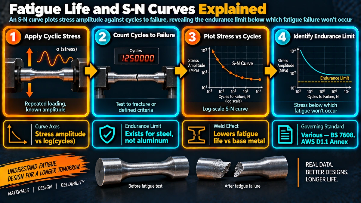
Fatigue failure occurs under repeated (cyclic) loading at stress levels that would cause no damage under a single static application — often well below the material’s yield strength. It proceeds in three recognizable stages: crack initiation at a stress concentration or microstructural defect, crack propagation as the flaw grows a small increment with each load cycle, and final fracture once the remaining cross-section can no longer support the applied load. The S-N curve addresses the combined initiation-plus-propagation life to failure as a single number for a given stress level, rather than separately quantifying each stage.
The Wöhler Curve and the S-N Curve
August Wöhler’s 19th-century testing of railway axles established the first systematic relationship between applied stress amplitude and the number of cycles to failure, and the resulting curve — plotting stress amplitude (S) against cycles to failure (N) on log-log axes — remains the standard fatigue design tool today. Strictly, the Wöhler curve spans the entire fatigue life range from low-cycle to high-cycle behavior, while the term “S-N curve” more specifically describes the elastic-dominated, high-cycle portion of that same relationship, where plastic strain per cycle is negligible and stress amplitude alone predicts life reliably. In practice the two terms are used interchangeably in most engineering contexts.
Low-Cycle vs High-Cycle Fatigue
| Regime | Typical Cycle Range | Dominant Strain Type | Analysis Method |
|---|---|---|---|
| Low-cycle fatigue (LCF) | Below ~10^4-10^5 cycles | Significant plastic strain per cycle | Strain-life (E-N), Coffin-Manson relationship |
| High-cycle fatigue (HCF) | Above ~10^5 cycles | Predominantly elastic strain | Stress-life (S-N) |
Most structural and pressure equipment fatigue design — including the weld joint fatigue classes covered in the WeldFabWorld fatigue-critical components guide — operates in the high-cycle regime where the standard stress-life S-N approach is appropriate. Low-cycle fatigue analysis, using strain rather than stress as the controlling parameter, becomes necessary for components experiencing large, infrequent stress cycles that produce meaningful plastic strain each time — thermal cycling of pressure equipment through startup/shutdown is a common example.
The Basquin Equation
In the high-cycle region, the S-N relationship follows a power law known as the Basquin equation, which is exactly why S-N data plots as a straight line on log-log axes:
Stress Ratio (R) and Mean Stress Effects
Most published S-N curves are generated under fully reversed loading, where stress cycles equally between tension and compression around zero mean stress. The stress ratio R quantifies the actual loading condition:
Real service loading is frequently not fully reversed, and a non-zero mean (tensile) stress generally reduces fatigue life compared to a fully reversed cycle at the same stress amplitude — this is what mean stress correction methods are built to account for.
Mean Stress Correction: Goodman, Gerber, and Soderberg
| Method | Formula | Character |
|---|---|---|
| Soderberg | sigma_a/Se + sigma_m/Sy = 1 | Most conservative — uses yield strength |
| Goodman | sigma_a/Se + sigma_m/Su = 1 | Linear, most commonly used in general design |
| Gerber | sigma_a/Se + (sigma_m/Su)^2 = 1 | Parabolic, best fit to test data, least conservative |
How S-N Curves Are Actually Generated
Fatigue life at a fixed stress level shows substantial scatter between nominally identical specimens — often an order of magnitude or more — driven by microstructural variability, surface finish, and small differences in inclusion content or surface defects acting as crack initiation sites. Because of this scatter, S-N curves are built from multiple specimens tested at each of several stress levels, and endurance limit determination specifically often uses the staircase method, where each specimen’s stress level depends on whether the previous specimen survived or failed. Design S-N curves published in codes typically represent a statistically conservative lower bound — commonly a 95% survival probability curve — rather than a simple average of the raw test data.
Where This Connects to Welded Joint Design
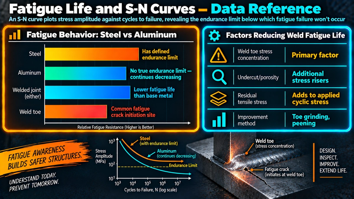
Everything above describes general S-N behavior for a smooth, unnotched specimen under a defined R-ratio. Welded joints break from this general framework in one specific, important way: fatigue design codes for welded structures (IIW, BS 7608, ASME Section VIII) assume worst-case, yield-magnitude tensile residual stress is always present at the weld toe in the as-welded condition, regardless of the applied load’s actual R-ratio. Because that assumption already represents close to the worst realistic mean stress condition, no additional Goodman-type mean stress benefit is permitted for as-welded joints — the full stress range, not stress amplitude corrected for mean stress, governs the applicable weld fatigue class. See the residual stress in welded joints guide for the mechanism behind that assumption and the fatigue-critical components guide for how weld joint classification actually works in practice.
Frequently Asked Questions
What is the difference between the Wohler curve and the S-N curve?
The terms are often used interchangeably, but strictly the Wohler curve describes fatigue behavior across the entire life range, from a fraction of a cycle through low-cycle fatigue and into high-cycle fatigue, while the S-N curve specifically describes the elastic-dominated, high-cycle region where plastic strain per cycle is negligible and stress amplitude alone can be related directly to cycles to failure. In practice, most engineering S-N curves published in codes and handbooks cover this high-cycle, stress-life region, since that is where the stress-life (S-N) approach is valid.
Why do ferrous metals have a true endurance limit but aluminum does not?
Ferrous metals, particularly steels, exhibit a fatigue mechanism related to dislocation locking by interstitial carbon and nitrogen atoms, which effectively arrests fatigue crack initiation below a certain stress amplitude, producing a true endurance limit — a stress below which the material can theoretically endure an infinite number of cycles without failure. Aluminum and most other non-ferrous alloys lack this locking mechanism, so their S-N curve continues sloping downward indefinitely rather than flattening out, which is why aluminum fatigue strength is always quoted at a specific number of cycles (commonly 10^8) rather than as a true infinite-life endurance limit.
What is the practical difference between low-cycle and high-cycle fatigue?
Low-cycle fatigue (LCF) involves relatively few cycles to failure, typically below about 10^4 to 10^5, with stress amplitudes high enough to cause significant plastic strain in each cycle, and is more accurately analyzed with the strain-life (E-N) approach using relationships such as the Coffin-Manson equation. High-cycle fatigue (HCF) involves a much larger number of cycles, with stress amplitudes low enough that deformation is predominantly elastic, and this is the regime where the standard stress-life (S-N) approach is valid and widely used in structural and mechanical design.
What does the R-ratio mean in fatigue testing and design?
The stress ratio R is the minimum stress divided by the maximum stress in a loading cycle (R = sigma_min / sigma_max). A fully reversed cycle, where the stress swings equally between tension and compression around zero mean stress, has R = -1 and is the baseline condition most published S-N curves are generated from. Real service loading often has a non-zero mean stress (R different from -1), which generally reduces fatigue life compared to a fully reversed cycle at the same stress amplitude, and this is exactly what mean stress correction methods like Goodman are used to account for.
Which mean stress correction method should be used: Goodman, Gerber, or Soderberg?
Soderberg is the most conservative of the three, using yield strength as the limiting value and generally underpredicting actual fatigue life by the widest margin. Goodman is a linear relationship using ultimate tensile strength and is the most commonly used method in general mechanical design because it offers a reasonable balance of conservatism and simplicity. Gerber uses a parabolic relationship that more closely fits actual test data for many ductile metals but is less conservative and less commonly specified in safety-critical codes as a result, since it allows a higher permissible alternating stress for a given mean stress than Goodman does.
Why do welded joint fatigue design codes not use Goodman or other mean stress corrections?
Codes governing welded joint fatigue design (IIW, BS 7608, ASME Section VIII) assume that worst-case, yield-magnitude tensile residual stress is always present at the weld toe in the as-welded condition, regardless of the applied load’s actual R-ratio, so the local stress at the crack initiation site effectively always cycles from a high tensile mean stress. Because this assumption already represents closer to the worst realistic case, no additional mean-stress benefit (such as a Goodman correction) is permitted for as-welded joints — see the WeldFabWorld residual stress and fatigue-critical components guides for how this plays out in weld-specific fatigue design class selection.
What is the Basquin equation and how is it used to describe an S-N curve mathematically?
The Basquin equation expresses the high-cycle fatigue region of the S-N curve as a power-law relationship, commonly written as stress amplitude = fatigue strength coefficient x (2N)^b, where N is cycles to failure and b is the fatigue strength exponent (typically a small negative number). This equation is why S-N data plots as a straight line on log-log axes in the high-cycle region — taking the logarithm of both sides of the power-law relationship produces a linear equation in log(stress) versus log(cycles), which is the standard way S-N data is presented and curve-fit in practice.
Why is scatter such a significant issue in fatigue testing, and how is it handled?
Fatigue life at a given stress level can vary by an order of magnitude or more between nominally identical specimens, driven by microstructural variability, surface finish differences, and small variations in inclusion content or surface defects that act as crack initiation sites. Because of this scatter, S-N curves are generated from multiple specimens tested at each stress level (or using methods like the staircase method specifically for endurance limit determination), and design S-N curves published in codes typically represent a statistically conservative lower bound (such as a 95% survival probability curve) rather than a simple average of the test data.
Recommended Reading
Metal Fatigue in Engineering (Stephens et al.)
Standard graduate-level reference on S-N, E-N, and fracture mechanics approaches to fatigue design.
View on AmazonMechanical Metallurgy (Dieter)
Covers fatigue mechanisms, S-N curve theory, and mean stress correction methods with worked examples.
View on AmazonFatigue of Structures and Materials (Schijve)
Comprehensive treatment of fatigue life prediction methods including Goodman, Gerber, and scatter analysis.
View on AmazonIIW Recommendations for Fatigue Design of Welded Joints
The reference standard for weld-specific fatigue classification building on the S-N fundamentals in this article.
View on AmazonDisclosure: WeldFabWorld participates in the Amazon Associates programme (StoreID: neha0fe8-21). If you purchase through these links, we may earn a small commission at no extra cost to you. This helps support free technical content on this site.